# Load packages for bivariate analysis workflow
if (!require("pacman")) install.packages("pacman")

pacman::p_load(
    sf,            # Spatial vector data handling
    terra,         # Modern raster data processing
    elevatr,       # Elevation data access
    cowplot,       # Plot composition tools
    geobr,
    censobr,
    dplyr,
    ggplot2,
    arrow
)Configuração
Instalação
Datasets disponíveis
# Available data sets
datasets <- list_geobr()
knitr::kable(head(datasets), row.names = FALSE)| function | geography | years | source |
|---|---|---|---|
read_country |
Country | 1872, 1900, 1911, 1920, 1933, 1940, 1950, 1960, 1970, 1980, 1991, 2000, 2001, 2010, 2013, 2014, 2015, 2016, 2017, 2018, 2019, 2020 | IBGE |
read_region |
Region | 2000, 2001, 2010, 2013, 2014, 2015, 2016, 2017, 2018, 2019, 2020 | IBGE |
read_state |
States | 1872, 1900, 1911, 1920, 1933, 1940, 1950, 1960, 1970, 1980, 1991, 2000, 2001, 2010, 2013, 2014, 2015, 2016, 2017, 2018, 2019, 2020 | IBGE |
read_meso_region |
Meso region | 2000, 2001, 2010, 2013, 2014, 2015, 2016, 2017, 2018, 2019, 2020 | IBGE |
read_micro_region |
Micro region | 2000, 2001, 2010, 2013, 2014, 2015, 2016, 2017, 2018, 2019, 2020 | IBGE |
read_intermediate_region |
Intermediate region | 2017, 2019, 2020 | IBGE |
Baixar uma área geográfica específica em um determinado ano
# State of Sergipe
state <- read_state(
  code_state="SE",
  year=2018,
  showProgress = FALSE
  )
mp1 <- ggplot() +
  geom_sf(data = state, color=NA, fill = 'lightblue') +
  theme_void()

# Municipality of Sao Paulo
muni <- read_municipality(
  code_muni = 3550308,
  year=2010,
  showProgress = FALSE
  )
mp2 <- ggplot() +
  geom_sf(data = muni, color=NA, fill = '#1ba185') +
  theme_void()

plot_grid(mp1, mp2, labels = c('Estado de Sergipe', 'Município de São Paulo'), label_size = 10)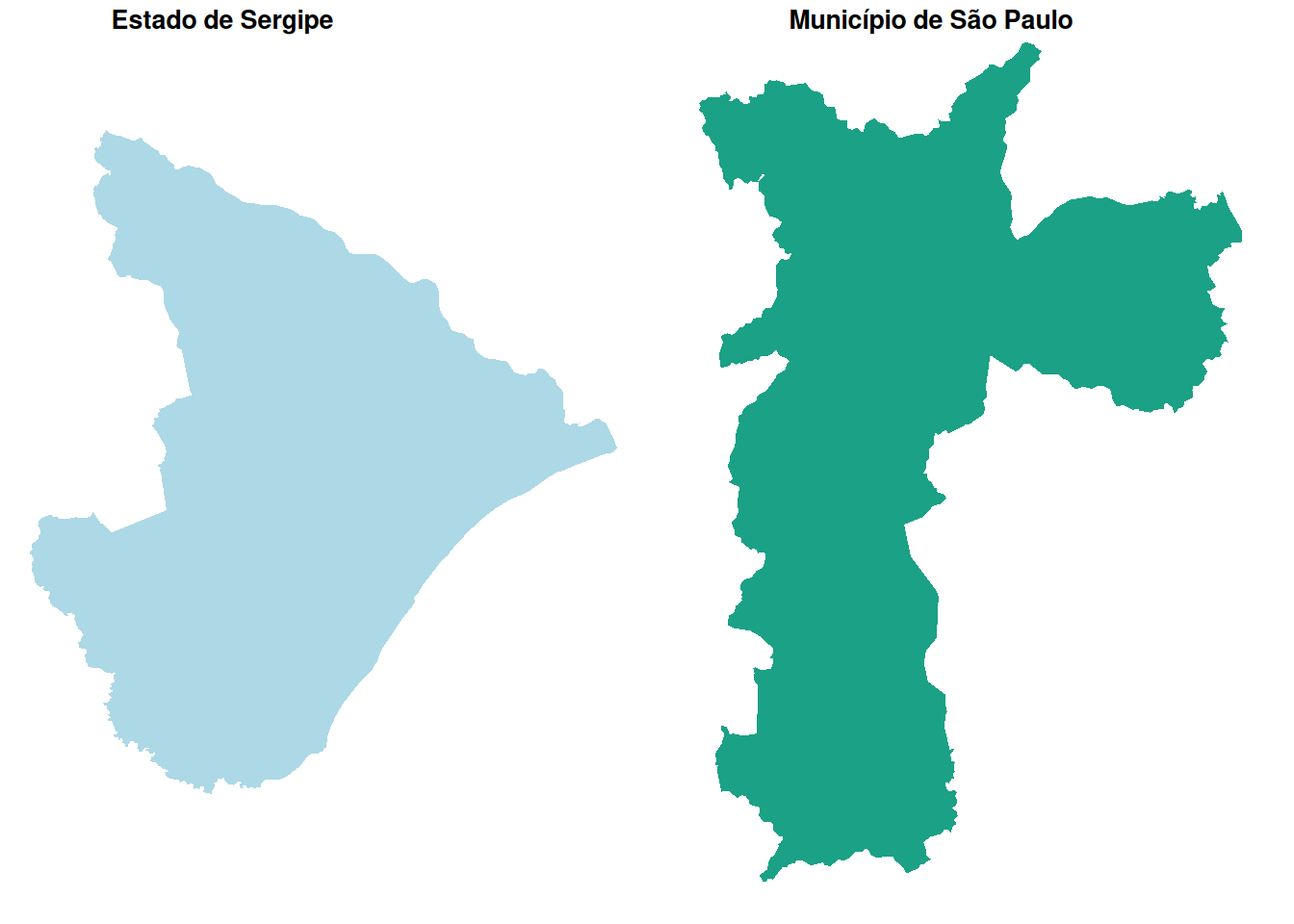
Baixar todas as áreas geográficas de um estado em um determinado ano
# All municipalities in the state of Minas Gerais
muni <- read_municipality(code_muni = "MG",
                          year = 2007,
                          showProgress = FALSE)
ggplot() +
  geom_sf(data=muni, fill="#2D3E50", color="#FEBF57", size=.15, show.legend = FALSE) +
  labs(subtitle="Municípios de Minas Gerais, 2007", size=8) +
  theme_minimal()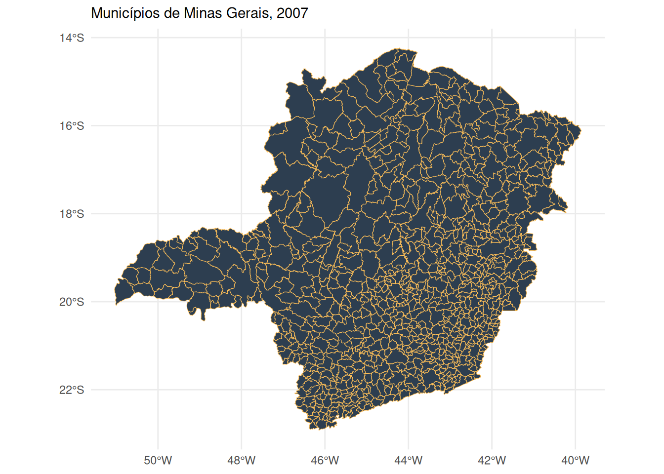
# All census tracts in the state of Rio de Janeiro
cntr <- read_census_tract(
  code_tract = "RJ",
  year = 2010,
  showProgress = FALSE
  )
head(cntr)
Simple feature collection with 6 features and 11 fields
Geometry type: MULTIPOLYGON
Dimension: XY
Bounding box: xmin: -42.1792 ymin: -22.9694 xmax: -42.0189 ymax: -22.9409
Geodetic CRS: SIRGAS 2000
code_tract zone code_muni name_muni name_neighborhood
1 330025805000046 URBANO 3300258 Arraial Do Cabo <NA>
2 330025805000047 URBANO 3300258 Arraial Do Cabo <NA>
3 330025805000048 URBANO 3300258 Arraial Do Cabo <NA>
4 330025805000049 URBANO 3300258 Arraial Do Cabo <NA>
5 330025805000050 URBANO 3300258 Arraial Do Cabo <NA>
6 330025805000051 URBANO 3300258 Arraial Do Cabo <NA>
code_neighborhood code_subdistrict name_subdistrict code_district
1 <NA> 33002580500 <NA> 330025805
2 <NA> 33002580500 <NA> 330025805
3 <NA> 33002580500 <NA> 330025805
4 <NA> 33002580500 <NA> 330025805
5 <NA> 33002580500 <NA> 330025805
6 <NA> 33002580500 <NA> 330025805
name_district code_state geom
1 Arraial Do Cabo 33 MULTIPOLYGON (((-42.0195 -2...
2 Arraial Do Cabo 33 MULTIPOLYGON (((-42.0228 -2...
3 Arraial Do Cabo 33 MULTIPOLYGON (((-42.1602 -2...
4 Arraial Do Cabo 33 MULTIPOLYGON (((-42.174 -22...
5 Arraial Do Cabo 33 MULTIPOLYGON (((-42.1759 -2...
6 Arraial Do Cabo 33 MULTIPOLYGON (((-42.1785 -2...Se o parâmetro code_ não for passado para a função, o geobr retornará os dados de todo o país por padrão.
# read all intermediate regions
inter <- read_intermediate_region(
  year = 2017,
  showProgress = FALSE
  )

# read all states
states <- read_state(
  year = 2019,
  showProgress = FALSE
  )

plot(states)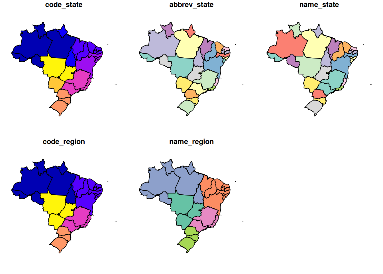
Depois de baixar os dados, é muito simples plotar mapas usando o ggplot2.
# Remove plot axis
no_axis <- theme(axis.title=element_blank(),
                 axis.text=element_blank(),
                 axis.ticks=element_blank())

# Plot all Brazilian states
ggplot() +
  geom_sf(data=states, fill="#2D3E50", color="#FEBF57", size=.15, show.legend = FALSE) +
  labs(subtitle="States", size=8) +
  theme_minimal() +
  no_axis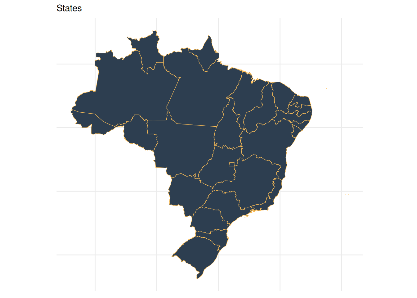
Trace todos os municípios de um determinado estado, como São Paulo:
# Download all municipalities
all_muni <- read_municipality(
  code_muni = "SP",
  year= 2010,
  showProgress = FALSE
  )

# plot
ggplot() +
  geom_sf(data=all_muni, fill="#2D3E50", color="#FEBF57", size=.15, show.legend = FALSE) +
  labs(subtitle="Municípios de São Paulo, 2010", size=8) +
  theme_minimal() +
  no_axis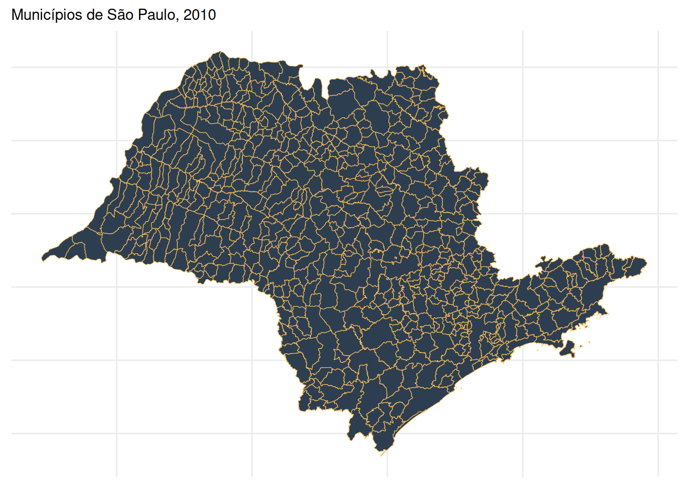
Mapas Temáticos
Unindo dados externos
# Read data.frame with life expectancy data
df <- utils::read.csv(system.file("extdata/br_states_lifexpect2017.csv", package = "geobr"), encoding = "UTF-8")

states$name_state <- tolower(states$name_state)
df$uf <- tolower(df$uf)

# join the databases
states <- dplyr::left_join(states, df, by = c("name_state" = "uf"))

ggplot() +
  geom_sf(data=states, aes(fill=ESPVIDA2017), color= NA, size=.15) +
    labs(subtitle="Atlas do Desenvolvimento Humano no Brasil. Pnud Brasil, Ipea e FJP, 2022", size=8) +
    scale_fill_distiller(palette = "Blues", name="Expectativa de vida ao nascer\n2017", limits = c(65,80)) +
    theme_minimal() +
    no_axis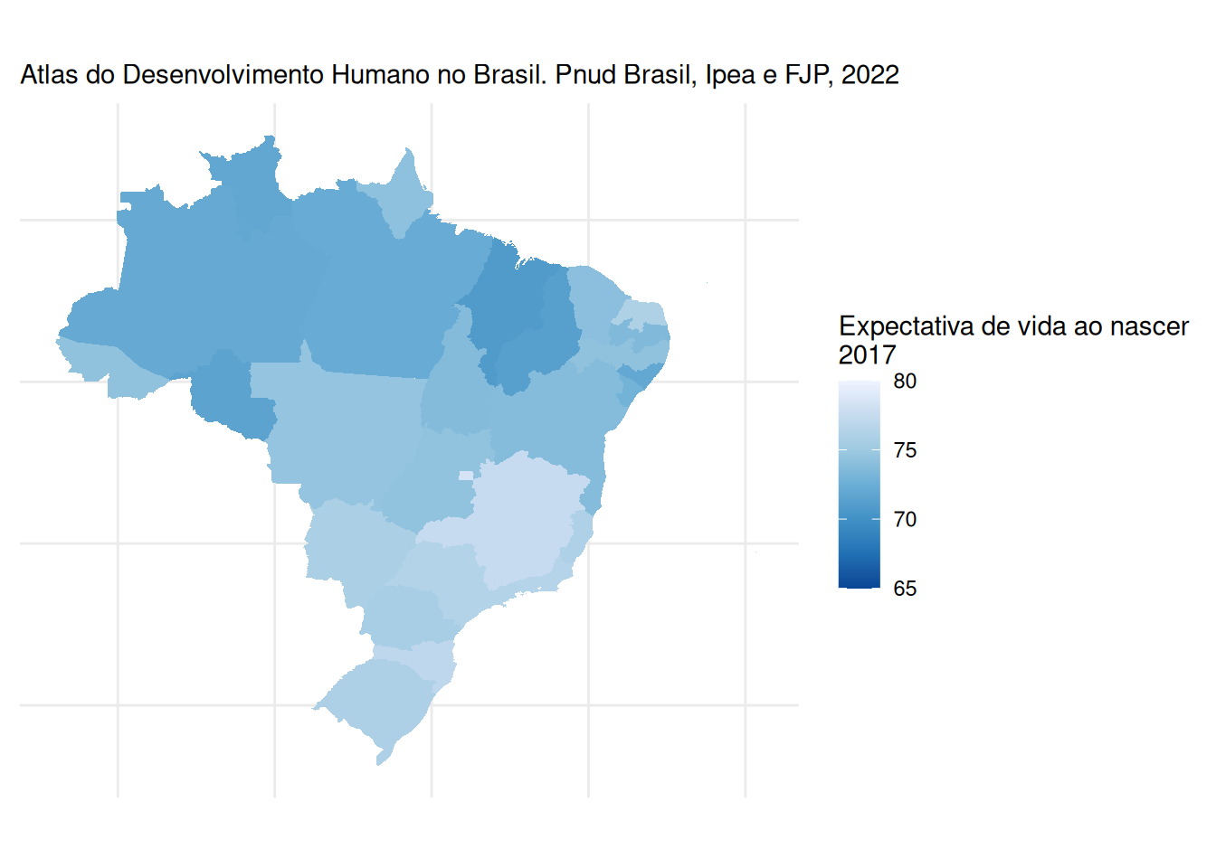
Usando o geobr junto com o censobr
# First, we need to download households data from the Brazilian census using the read_households() function.
hs <- read_households(year = 2010,
                      showProgress = FALSE)
# Now we’re going to (a) group observations by municipality, (b) get the number of households connected to a sewage network, (c) calculate the proportion of households connected, and (d) collect the results.
esg <- hs |>
        collect() |>
        group_by(code_muni) |>                                             # (a)
        summarize(rede = sum(V0010[which(V0207=='1')]),                    # (b)
                  total = sum(V0010)) |>                                   # (b)
        mutate(cobertura = rede / total) |>                                # (c)
        collect()                                                          # (d)
knitr::kable(head(esg), row.names = FALSE)
Agora só precisamos baixar as geometrias dos municípios brasileiros do geobr, unir os dados espaciais com nossas estimativas e mapear os resultados.
# download municipality geometries
muni_sf <- geobr::read_municipality(year = 2010,
                                    showProgress = FALSE)
#> Using year/date 2010

# merge data
esg_sf <- left_join(muni_sf, esg, by = 'code_muni')

# plot map
ggplot() +
  geom_sf(data = esg_sf, aes(fill = cobertura), color=NA) +
  labs(title = "Proporção de domicílios conectados a uma rede de esgoto (Censo 2010)") +
  scale_fill_distiller(palette = "Greens", direction = 1,
                       name='Proporção de\ndomicílios',
                       labels = scales::percent) +
  theme_void()
Referências
- geobr: Download Official Spatial Data Sets of Brazil https://ipeagit.github.io/geobr
- Introduction to geobr (R) https://cran.r-project.org/web/packages/geobr/vignettes/intro_to_geobr.html
- Atlas do Desenvolvimento Humano no Brasil. Pnud Brasil, Ipea e FJP, 2022 http://www.atlasbrasil.org.br/consulta/planilha
Copyright
Geosaber₢2025